分类法/范例一: Recognizing hand-written digits
http://scikit-learn.org/stable/auto_examples/classification/plot_digits_classification.html
这个范例用来展示scikit-learn 机器学习套件,如何用SVM演算法来达成手写的数字辨识
- 利用
make_classification建立模拟资料 - 利用
sklearn.datasets.load_digits()来读取内建资料库 - 用线性的SVC来做分类,以8x8的影像之像素值来当作特徵(共64个特徵)
- 用
metrics.classification_report来提供辨识报表
(一)引入函式库及内建手写数字资料库
引入之函式库如下
- matplotlib.pyplot: 用来绘製影像
- sklearn.datasets: 用来绘入内建之手写数字资料库
- sklearn.svm: SVM 支持向量机之演算法物件
- sklearn.metrics: 用来评估辨识准确度以及报表的显示
import matplotlib.pyplot as plt
from sklearn import datasets, svm, metrics

# The digits dataset
digits = datasets.load_digits()
使用datasets.load_digits()将资料存入,digits为一个dict型别资料,我们可以用以下指令来看一下资料的内容。
for key,value in digits.items() :
    try:
        print (key,value.shape)
    except:
        print (key)
| 显示 | 说明 |
|---|---|
| ('images', (1797L, 8L, 8L)) | 共有 1797 张影像,影像大小为 8x8 |
| ('data', (1797L, 64L)) | data 则是将8x8的矩阵摊平成64个元素之一维向量 |
| ('target_names', (10L,)) | 说明10种分类之对应 [0, 1, 2, 3, 4, 5, 6, 7, 8, 9] |
| DESCR | 资料之描述 |
| ('target', (1797L,)) | 记录1797张影像各自代表那一个数字 |
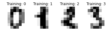
接下来我们试著以下面指令来观察资料档,每张影像所对照的实际数字存在digits.target变数中
images_and_labels = list(zip(digits.images, digits.target))
for index, (image, label) in enumerate(images_and_labels[:4]):
    plt.subplot(2, 4, index + 1)
    plt.axis('off')
    plt.imshow(image, cmap=plt.cm.gray_r, interpolation='nearest')
    plt.title('Training: %i' % label)
(二)训练以及分类
接下来的步骤则是使用reshape指令将8x8的影像资料摊平成64x1的矩阵。
接著用classifier = svm.SVC(gamma=0.001)产生一个SVC分类器(Support Vector Classification)。再将一半的资料送入分类器来训练classifier.fit(资料:898x64, 分类目标:898x1)。SVC之预设kernel function为RBF (radial basis function):  . 其中
. 其中SVC(gamma=0.001)就是在设定RBF函数里的 这个值必需要大于零。最后,再利用后半部份的资料来测试训练完成之SVC分类机
predict(data[n_samples / 2:])将预测结果存入predicted变数,而原先的真实目标资料则存于expected变数,用于下一节之准确度统计。
n_samples = len(digits.images)

# 资料摊平:1797 x 8 x 8 -> 1797 x 64
# 这里的-1代表自动计算,相当于 (n_samples, 64)
data = digits.images.reshape((n_samples, -1))

# 产生SVC分类器
classifier = svm.SVC(gamma=0.001)

# 用前半部份的资料来训练
classifier.fit(data[:n_samples / 2], digits.target[:n_samples / 2])

expected = digits.target[n_samples / 2:]

#利用后半部份的资料来测试分类器,共 899笔资料
predicted = classifier.predict(data[n_samples / 2:])
若是观察 expected 及 predicted 矩阵中之前10个变数可以得到:
expected[:10]:[8 8 4 9 0 8 9 8 1 2]predicted[:10]:[8 8 4 9 0 8 9 8 1 2]
这说明了前10个元素中,我们之前训练完成的分类机,正确的分类了手写数字资料。那对于全部测试资料的准确度呢?要如何量测?
(三)分类准确度统计
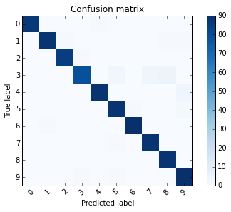
那在判断准确度方面,我们可以使用一个名为「混淆矩阵」(Confusion matrix)的方式来统计。
print("Confusion matrix:\n%s"
    % metrics.confusion_matrix(expected, predicted))
使用sklearn中之metrics物件,metrics.confusion_matrix(真实资料:899, 预测资料:899)可以列出下面矩阵。此矩阵对角线左上方第一个数字 87,代表实际为0且预测为0的总数有87个,同一列(row)第五个元素则代表,实际为0但判断为4的资料个数为1个。
Confusion matrix:
[[87  0  0  0  1  0  0  0  0  0]
 [ 0 88  1  0  0  0  0  0  1  1]
 [ 0  0 85  1  0  0  0  0  0  0]
 [ 0  0  0 79  0  3  0  4  5  0]
 [ 0  0  0  0 88  0  0  0  0  4]
 [ 0  0  0  0  0 88  1  0  0  2]
 [ 0  1  0  0  0  0 90  0  0  0]
 [ 0  0  0  0  0  1  0 88  0  0]
 [ 0  0  0  0  0  0  0  0 88  0]
 [ 0  0  0  1  0  1  0  0  0 90]]
我们可以利用以下的程式码将混淆矩阵图示出来。由图示可以看出,实际为3时,有数次误判为5,7,8。
def plot_confusion_matrix(cm, title='Confusion matrix', cmap=plt.cm.Blues):
    import numpy as np
    plt.imshow(cm, interpolation='nearest', cmap=cmap)
    plt.title(title)
    plt.colorbar()
    tick_marks = np.arange(len(digits.target_names))
    plt.xticks(tick_marks, digits.target_names, rotation=45)
    plt.yticks(tick_marks, digits.target_names)
    plt.tight_layout()
    plt.ylabel('True label')
    plt.xlabel('Predicted label')

plt.figure()
plot_confusion_matrix(metrics.confusion_matrix(expected, predicted))
以手写影像3为例,我们可以用四个数字来探讨判断的精准度。
- True Positive(TP,真阳):实际为3且判断为3,共79个
- False Positive(FP,伪阳):判断为3但判断错误,共2个
- False Negative(FN,伪阴):实际为3但判断错误,共12个
- True Negative(TN,真阴):实际不为3,且判断正确。也就是其馀899-79-2-12=885个
而在机器学习理论中,我们通常用以下precision, recall, f1-score来探讨精确度。以手写影像3为例。
- precision = TP/(TP+FP) = 79/81 = 0.98
- 判断为3且实际为3的比例为0.98
- recall = TP/(TP+FN) = 79/91 = 0.87
- 实际为3且判断为3的比例为0.87
- f1-score 则为以上两者之「harmonic mean 调和平均数」
- f1-score= 2 x precision x recall/(recision + recall) = 0.92
metrics物件里也提供了方便的函式metrics.classification_report(expected, predicted)计算以上统计数据。
print("Classification report for classifier %s:\n%s\n"
    % (classifier, metrics.classification_report(expected, predicted)))
此报表最后的 support,则代表著实际为手写数字的总数。例如实际为3的数字共有91个。
             precision    recall  f1-score   support

          0       1.00      0.99      0.99        88
          1       0.99      0.97      0.98        91
          2       0.99      0.99      0.99        86
          3       0.98      0.87      0.92        91
          4       0.99      0.96      0.97        92
          5       0.95      0.97      0.96        91
          6       0.99      0.99      0.99        91
          7       0.96      0.99      0.97        89
          8       0.94      1.00      0.97        88
          9       0.93      0.98      0.95        92

avg / total       0.97      0.97      0.97       899
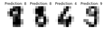
最后,用以下的程式码可以观察测试影像以及预测(分类)结果得对应关系。
images_and_predictions = list(
                        zip(digits.images[n_samples / 2:], predicted))
for index, (image, prediction) in enumerate(images_and_predictions[:4]):
    plt.subplot(2, 4, index + 5)
    plt.axis('off')
    plt.imshow(image, cmap=plt.cm.gray_r, interpolation='nearest')
    plt.title('Prediction: %i' % prediction)

plt.show()
(四)完整程式码
Python source code: plot_digits_classification.py
http://scikit-learn.org/stable/_downloads/plot_digits_classification.py
print(__doc__)

# Author: Gael Varoquaux <gael dot varoquaux at normalesup dot org>
# License: BSD 3 clause

# Standard scientific Python imports
import matplotlib.pyplot as plt

# Import datasets, classifiers and performance metrics
from sklearn import datasets, svm, metrics

# The digits dataset
digits = datasets.load_digits()

# The data that we are interested in is made of 8x8 images of
# digits, let's # have a look at the first 3 images, stored in
# the `images` attribute of the # dataset.  If we were working
# from image files, we could load them using # pylab.imread.
# Note that each image must have the same size. For these  images,
#we know which digit they represent: it is given in the 'target' of
# the dataset.
images_and_labels = list(zip(digits.images, digits.target))
for index, (image, label) in enumerate(images_and_labels[:4]):
    plt.subplot(2, 4, index + 1)
    plt.axis('off')
    plt.imshow(image, cmap=plt.cm.gray_r, interpolation='nearest')
    plt.title('Training: %i' % label)

# To apply a classifier on this data, we need to flatten the image, to
# turn the data in a (samples, feature) matrix:
n_samples = len(digits.images)
data = digits.images.reshape((n_samples, -1))

# Create a classifier: a support vector classifier
classifier = svm.SVC(gamma=0.001)

# We learn the digits on the first half of the digits
classifier.fit(data[:n_samples / 2], digits.target[:n_samples / 2])

# Now predict the value of the digit on the second half:
expected = digits.target[n_samples / 2:]
predicted = classifier.predict(data[n_samples / 2:])

print("Classification report for classifier %s:\n%s\n"
    % (classifier, metrics.classification_report(expected, predicted)))
print("Confusion matrix:\n%s"
    % metrics.confusion_matrix(expected, predicted))

images_and_predictions = list(
                        zip(digits.images[n_samples / 2:], predicted))
for index, (image, prediction) in enumerate(images_and_predictions[:4]):
    plt.subplot(2, 4, index + 5)
    plt.axis('off')
    plt.imshow(image, cmap=plt.cm.gray_r, interpolation='nearest')
    plt.title('Prediction: %i' % prediction)

plt.show()